Generalization and Compression
…work in progress…
Intro
This piece was inspired by the paper “Understanding deep learning requires rethinking generalization” by Zhang and colleagues (2016). The paper states that under the generalization conditions established by the classical generalization theories (VC and Radamacher, …) – namely that the capacity of the model classes must be reasonably constrained, in other word able to learn only a limited number of ways the data can be split between two target classes – the deep learning models that generalize perfectly well are not guaranteed to do so.
Experiment with random data: random labelling induces nowhere differentiable loss function. Fat Cantor set?
Compression: an empirical study
On intuition level, learning representations goes together with compression of data.
If we assume data is ‘meaninful’ or not arbitrary random, which we can more precisely formulate as data having low Kolmogorov complexity. Pragmatically speaking we expect the data to be compressible.
Compression in context of neural networks has been extensively discussed for the case of autoencoders. Unlike generative autoencoders, we are dealing with a discriminative model here, so some additional explanation might be needed. However for now we take an intuitive assumption that learning discriminative mapping also induces compression of the feature vectors by the network.
Therefore, using the framework of fitting the random data suggested by Zhang et al. (2016) I explored compression in a ReLU CNN network on MNIST.
Model in keras
def build_model():
    model = Sequential()

    # LAYER 0
    model.add(Convolution2D(nb_filters, kernel_size[0], kernel_size[1],
                            border_mode='valid',
                            input_shape=input_shape))
    # LAYER 1
    model.add(Activation('relu'))
    # LAYER 2
    model.add(Convolution2D(nb_filters, kernel_size[0], kernel_size[1]))
    # LAYER 3
    model.add(Activation('relu'))
    # LAYER 4
    model.add(MaxPooling2D(pool_size=pool_size))
    # LAYER 5
    model.add(Dropout(0.25))
    # LAYER 6
    model.add(Flatten())
    # LAYER 7
    model.add(Dense(128))
    # LAYER 8
    model.add(Activation('relu'))
    # LAYER 9
    model.add(Dropout(0.5))
    # LAYER 10
    model.add(Dense(nb_classes))
    # LAYER 11
    model.add(Activation('softmax'))

    return model
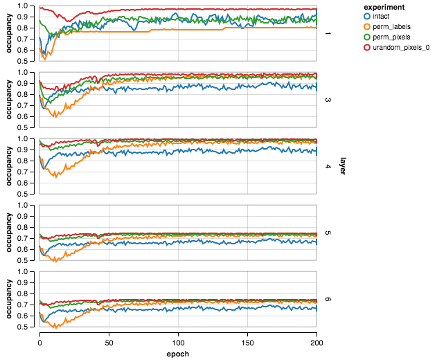
I picked ReLU activation as it causes some of the hidden nodes to have zero activation (those that have a negative pre-ReLU input). This gives a simple proxy for the information and entropy per layer: occupancy (proportion of non-zero activations within the layer).
 |
In this picture I included only those layers that display some (variable) degree of sparsity. Four data corruption experiments are shown:
intact– standard MNIST (4000 samples)perm_labels– permuted labelsperm_pixels– permuted pixelsurand_pixels_0– uniform random pixels
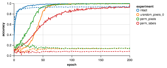
One can see that the occupancy in the intact case (in blue) is lowest (except first layer), corroborating the assumption that the intact data is the most compressible. Moreover, judging from the graph below, the occupancy / accuracy ratio is most efficient (lowest) for intact data.
 |
 |
The figure above is a sanity check, analoguous to Fig.1a in Zhang et al., 2016.
Thoughts
Correlation between $x_1$ and $x_2$ -> weights learn to reflect joint probability $P(x_1, x_2)$ ->
Why weights do not learn more complex structures than necessary? Is it in any sense more expensive or less probable?
Can we formulate generalization in terms of probability of difference between two empirical probabilities?
\[\int_w P(w(\{x\}^{(0)})) [log P^{(0)}(y|x) - log P^{(0)}(y|x)]\]